
 I have been busy attending conferences recently (one of many excuses for not updating the blog) and I thought I would mention one significant difference between these conferences and those that I have attended previously. At Behaviour 2013 (Newcastle, 4-8 Aug 2013 – that’s me talking about mimicry on the right), I tried live-tweeting for the first time. Then at Intecol 2013 (London, 18-23 Aug 2013) almost all questions during the plenary talks were taken solely by Twitter. This meant that I had a lot more experience of Twitter in an academic forum that I had had before, and I found it to be an immensely positive experience! Not only did people come up and say “hi” because they recognised my name from Twitter (new networking opportunities), but I passively participated in multiple parallel sessions where usually I would only have had access to the session within which I was physically present (there were 16 parallel sessions at any one time at Intecol!).
When I got back, I was interested to see how many people were engaging – is it just a few nerds, or is there a wider move towards social media in research? I put together some R code to analyse the tweets from Wednesday 21st August at Intecol and the European Society for Evolutionary Biology (ESEB) meeting that was happening at the same time (I picked this day because both conferences were running regular, full-day talks, and the tweets are still available to the Twitter API). This is the first time I have tried accessing an API through Twitter, and it wasn’t entirely straightforward so I have posted the code below in case anyone else wants to try it. The code assumes that you have already authenticated using OAuth (see here for a guide) and the backbone was provided by a post on R-Bloggers. I know that there were 1491 delegates at ESEB and around 2000 at Intecol, so bear in mind the difference in attendance when interpreting these figures:
Tweets sent on 21st August:
– ESEB: 584
– Intecol: 2251
Unique Twitter users engaged on 21st August:
– ESEB: 98
– Intecol: 539
For those of you who are interested, here are the timelines of activity (note the variation in scale on the y-axis):
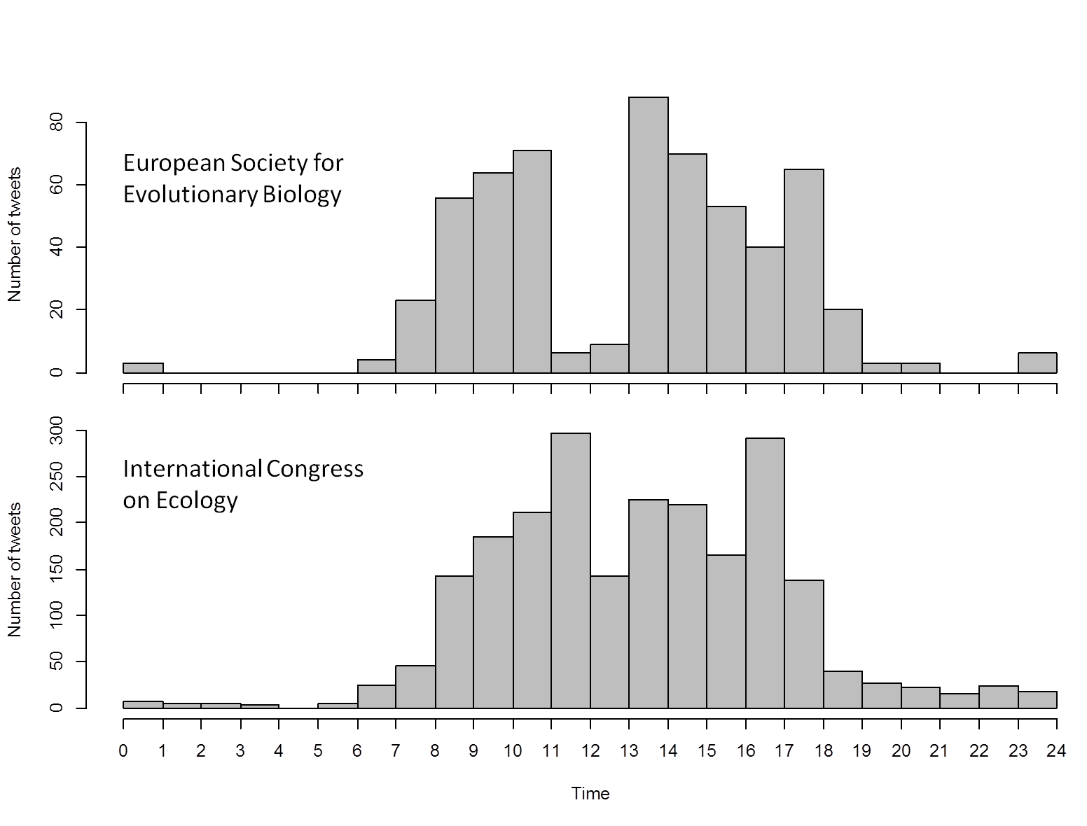
What you can see is that there are distinct peaks at Intecol around 11am (the BES Presidential Address by Georgina Mace) and 4pm (which was a provocative plenary about policy and science featuring some big names, including Bob May and John Lawton). Intecol pursued a fairly aggressive policy of Twitter use, incorporating it into the official talks as well as promoting its use at every opportunity. The result was a huge amount of engagement from people, and a great deal of discussion about its merits (and demerits, from some quarters!). I’d be interested to hear whether the ESEB peaks and troughs can be explained? I assume that they coincide with plenaries as well?
Some closing thoughts:
- Aggressive Twitter promotion was successful at Intecol, providing huge engagement, but not popular with all attendees.
- Having Twitter usernames on name badges is a must if this is going to be a key way of interacting with fellow attendees.
- In particular, the use of Twitter for questions in plenaries was an EXCELLENT idea, keeping questions brief and focused, while removing concerns over anxiety about publicly getting up to the microphone.
- Live discussion within the community during the plenaries was fascinating as well – people provided links to papers that were cited, questioned assumptions, and even provided cricket scores!
NB: Because tweets become inaccessible via the Twitter API after 5-6 days, here are the tweets from that day for posterity: ESEB and Intecol Tweets.
# Based on http://www.r-bloggers.com/visualising-activity-around-a-twitter-hashtag-or-search-term-using-r/
# Load the twitteR package
library (twitteR)
# You will need this file from the previous link, created using oauth
load("twitteR_credentials")
registerTwitterOAuth(twitCred)
# These searches simply reach back and pull out tweets by looking for the hashtags of the two conferences for a specific day
IntecolTweets <- searchTwitter("#int13", n=5000,cainfo="cacert.pem",since='2013-08-21', until='2013-08-22')
ESEBTweets <- searchTwitter("#eseb2013", n=2500,cainfo="cacert.pem",since='2013-08-21', until='2013-08-22')
#Make use of a handy dataframe creating twitteR helper function
IntecolTweets.df=twListToDF(IntecolTweets)
ESEBTweets.df=twListToDF(ESEBTweets)
# To plot the data, I was working with simple forms of the dates (in seconds) - these come in useful in a minute
starttime <- strptime("2013-08-21 00:00:00","%Y-%m-%d %H:%M:%S", tz = "UTC")
endtime <- strptime("2013-08-22 00:00:00","%Y-%m-%d %H:%M:%S", tz = "UTC")
# Creating bins for plotting
timepoints<-seq(from=as.double(starttime),to=as.double(endtime),length.out=25)
timelabels<-seq(0,24,length.out=25)
# Plot settings
par(mfrow=c(2,1))
hist(as.double(ESEBTweets.df$created),breaks=timepoints,main=NA,xlab="Time",ylab="Number of tweets",xaxt="n",col="grey")
axis(side=1,at=timepoints,labels=timelabels)
hist(as.double(IntecolTweets.df$created),breaks=timepoints,main=NA,xlab="Time",ylab="Number of tweets",xaxt="n",col="grey")
axis(side=1,at=timepoints,labels=timelabels)
